Evanston Restaurant Food Violations
Patrick Tu
2022-08-28
For our next R analysis I decided to focus on the town where we live, Evanston. We decided to analyze which restaurants in Evanston had the most food violations and map the data.
One thing to note about this data is it is from 2018-2019 and some of the restaurants mapped are no longer open. Here’s the link for the violations data and the restaurants data we used for this analysis.
library(ggmap)
library(tidyverse)
library(osmdata)
library(sf)
library(plotly)
# Data sets for project
restaurants <-
read_csv(file = "Data/Evanston_restaurants.csv") %>%
select(
business_license = `Business License`,
business_name = `Business Name`,
address = Address,
city = City,
state = State,
zip = `Zip Code`,
location = Location,
last_inspection = `Last Inspection Date`
) %>%
mutate(last_inspection = as.Date(last_inspection, format = "%m/%d/%Y")) %>%
separate(location, into = c("location", "lat"), sep = "\\(") %>%
separate(lat, into = c("lat", "long"), sep = ",") %>%
mutate(long = gsub("\\)", "", long),
long = as.numeric(long),
lat = as.numeric(lat))
violations <-
read_csv(file = "Data/Evanston_restaurant_violations.csv") %>%
select(
business_license = `Business LIcense`,
violation_date = `Violation Date`,
violation = Violation,
comments = `Inspector Comments`
) %>%
mutate(violation_date = as.Date(violation_date, format = "%m/%d/%Y"))
violation_data <- left_join(violations, restaurants, by = "business_license")# Code inspired by Mark Padgham and Robin Lovelace(https://cran.r-project.org/web/packages/osmdata/vignettes/osmdata.html)
# Evanston
coords <- matrix(c(-87.7324, -87.6623, 42.0189, 42.0714),
byrow = TRUE, nrow = 2,
ncol = 2,
dimnames = list(c('x','y'),
c('min','max')))
location <- coords %>% opq()#build different types of streets
main_st <-
data.frame(
type = c(
"motorway",
"trunk",
"primary",
"motorway_junction",
"trunk_link",
"primary_link",
"motorway_link"
)
)
st <- data.frame(type = available_tags('highway'))
st <- subset(st, !type %in% main_st$type)
path <- data.frame(type = c("footway","path","steps","cycleway"))
st <- subset(st, !type %in% path$type)
st <- as.character(st$type)
main_st <- as.character(main_st$type)
path <- as.character(path$type)
#query OSM
main_streets <-
location %>%
add_osm_feature(key = "highway", value = main_st) %>%
osmdata_sf()
streets <-
location %>%
add_osm_feature(key = "highway", value = st) %>%
osmdata_sf()
water <-
location %>%
add_osm_feature(key = "natural", value = c("water")) %>%
osmdata_sf()
rail <-
location %>%
add_osm_feature(key = "railway", value = c("rail")) %>%
osmdata_sf()
parks <-
location %>%
add_osm_feature(
key = "leisure",
value = c(
"park",
"nature_reserve",
"recreation_ground",
"golf_course",
"pitch",
"garden"
)
) %>%
osmdata_sf()Here we mapped all restaurants in Evanston in 2019. As you can see there are several clusters of restaurants most notably the downtown area near the center of the map.
#plot map
evanston_map <- ggplot() +
  geom_sf(data = parks$osm_polygons, fill = '#94ba8e') +
  geom_sf(data = water$osm_polygons, fill = '#c6e1e3') +
  geom_sf(data = water$osm_multipolygons, fill = '#c6e1e3') +
  geom_sf(data = streets$osm_lines, size = 0.75, color = '#eedede') +
  geom_sf(data = main_streets$osm_lines, color = '#ff9999', size = 0.5) +
  geom_sf(data = rail$osm_lines, color = '#596060', size = 1) +
  geom_point(data = restaurants, size = 0.5, aes(x = long, y = lat))+
  coord_sf(
    xlim = c(coords[1], coords[1,2]),
    ylim = c(coords[2], coords[2,2]),
    expand = TRUE
  ) +
  theme_minimal()
evanston_map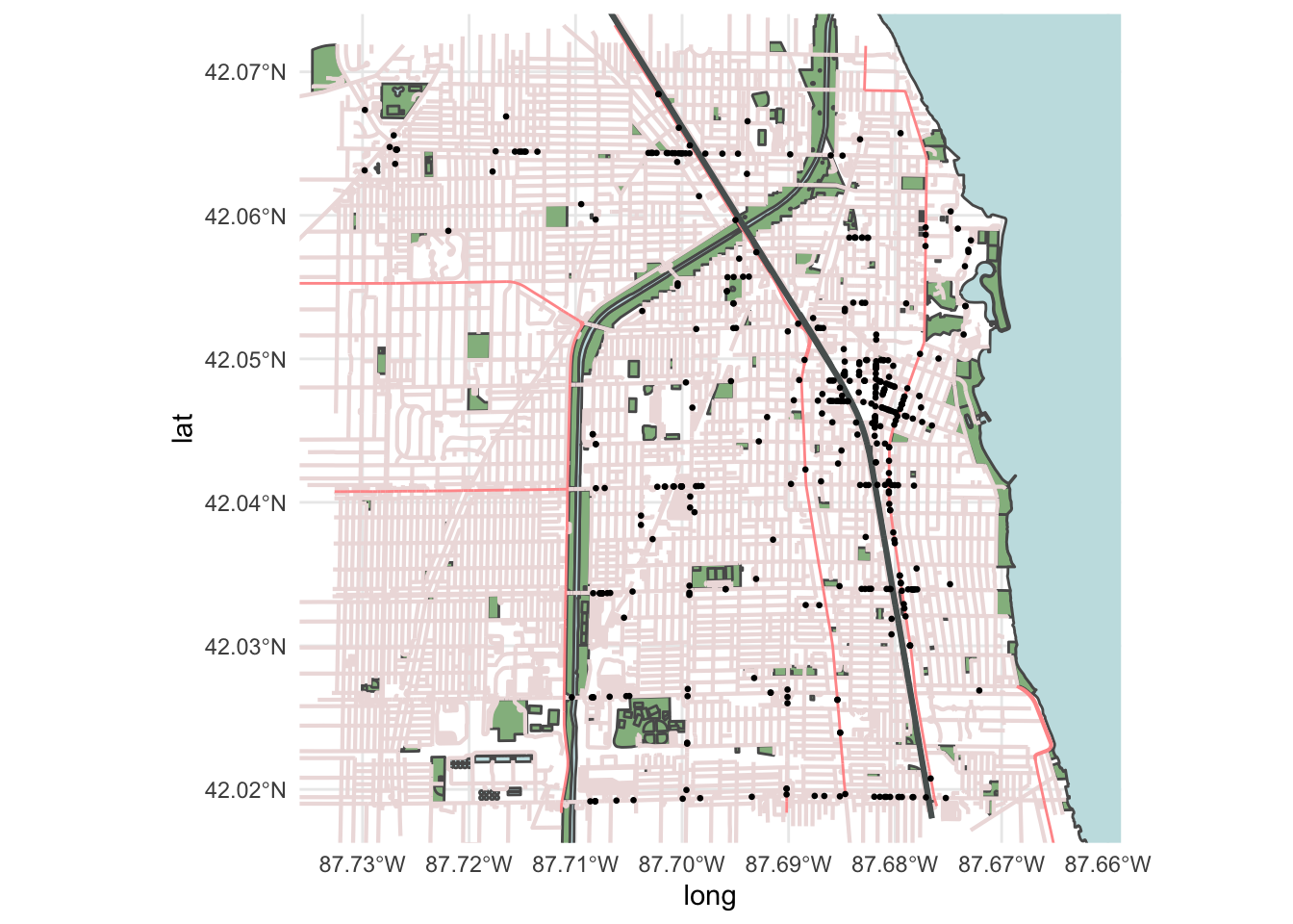
We noticed most restaurants in Evanston had two or less critical food violations so we decided that we would plot all of the restaurants with three or more critical violations. We decided to create a bar graph of which violations were the most common before plotting the data on the map.
freq_vio <- violation_data %>%
  select(violation, comments, business_name, lat, long) %>%
  mutate(
    violation_num = regmatches(
      violation,
      gregexpr("[[:digit:]]{1,2}", violation)
    ),
    violation_num = as.numeric(violation_num),
    crit_vio = grepl("CRITICAL VIOLATION", comments)
  )

freq_vio_sum <- freq_vio %>%
  count(violation_num)

ggplot(data = freq_vio_sum,
         aes(x = reorder(violation_num,n),  y = n))+
  geom_bar(stat = "identity")+
  #scale_x_continuous(breaks = seq(1,45,1), minor_breaks = NULL)+
  labs(
    title = "Bar Graph of City of Evanston Food Violations",
    x = "Violation Code",
    y = "Violations"
  )+
  coord_flip()
freq_res_vio <- freq_vio %>%
  count(business_name, crit_vio)

filter_vio <- filter(freq_res_vio, n > 2, crit_vio == TRUE)

three_vio_res <- filter(freq_vio,
                        business_name %in% filter_vio$business_name,
                        crit_vio == TRUE)
Next we created an interactive map of all the restaurants in Evanston with three or more critical violation. We used the package plotly for this.
merge_vio <-
  three_vio_res %>%
  group_by(business_name) %>%
  mutate(violations = toString(violation)) %>%
  mutate(violations = gsub("., ", "\r", violations, fixed = TRUE))

vio_merge_map <- ggplot() +
  geom_sf(data = parks$osm_polygons, fill = '#94ba8e') +
  geom_sf(data = water$osm_polygons, fill = '#c6e1e3') +
  geom_sf(data = water$osm_multipolygons, fill = '#c6e1e3') +
  geom_sf(data = streets$osm_lines, size = 0.75, color = '#eedede') +
  geom_sf(data = main_streets$osm_lines, color = '#ff9999', size = 0.5) +
  geom_sf(data = rail$osm_lines, color = '#596060', size = 1) +
  geom_point(data = merge_vio,
             size = 0.75, aes(
               x = long,
               y = lat,
               group = business_name, color = violations), alpha = 0.5)+
  scale_color_manual(values = rep("black", 49))+
  coord_sf(
    xlim = c(coords[1], coords[1,2]),
    ylim = c(coords[2], coords[2,2]),
    expand = TRUE
  ) +
  theme_minimal()+
  theme(
    legend.position = "none",
    axis.text = element_blank(),
    axis.title = element_blank()
  )

ggplotly(vio_merge_map)
As with the previous map the downtown area has the highest concentration of restaurants with critical violations. Each data point has the name of the business, violation, and coordinates listed. In the future we may do more data analysis projects that focus on Evanston.