NBA Player Comparison Function
Patrick Tu
5/28/2022
I developed a function that compares two players in the NBA using the nbastatR package. The function compares the players based on their advanced and/or per game statistics.
If you want to use this function it is on my github here is how you would source it onto your workspace.
Notes: If you want to use the function you will have to download the nbastatR, dplyr, ggplot2, tidyr, Hmisc, ghibli packages.
library(devtools)
source_url("https://raw.githubusercontent.com/pltu06/pltu06.github.io/main/NBA_player_function.R")
Here’s some different ways to use the function.
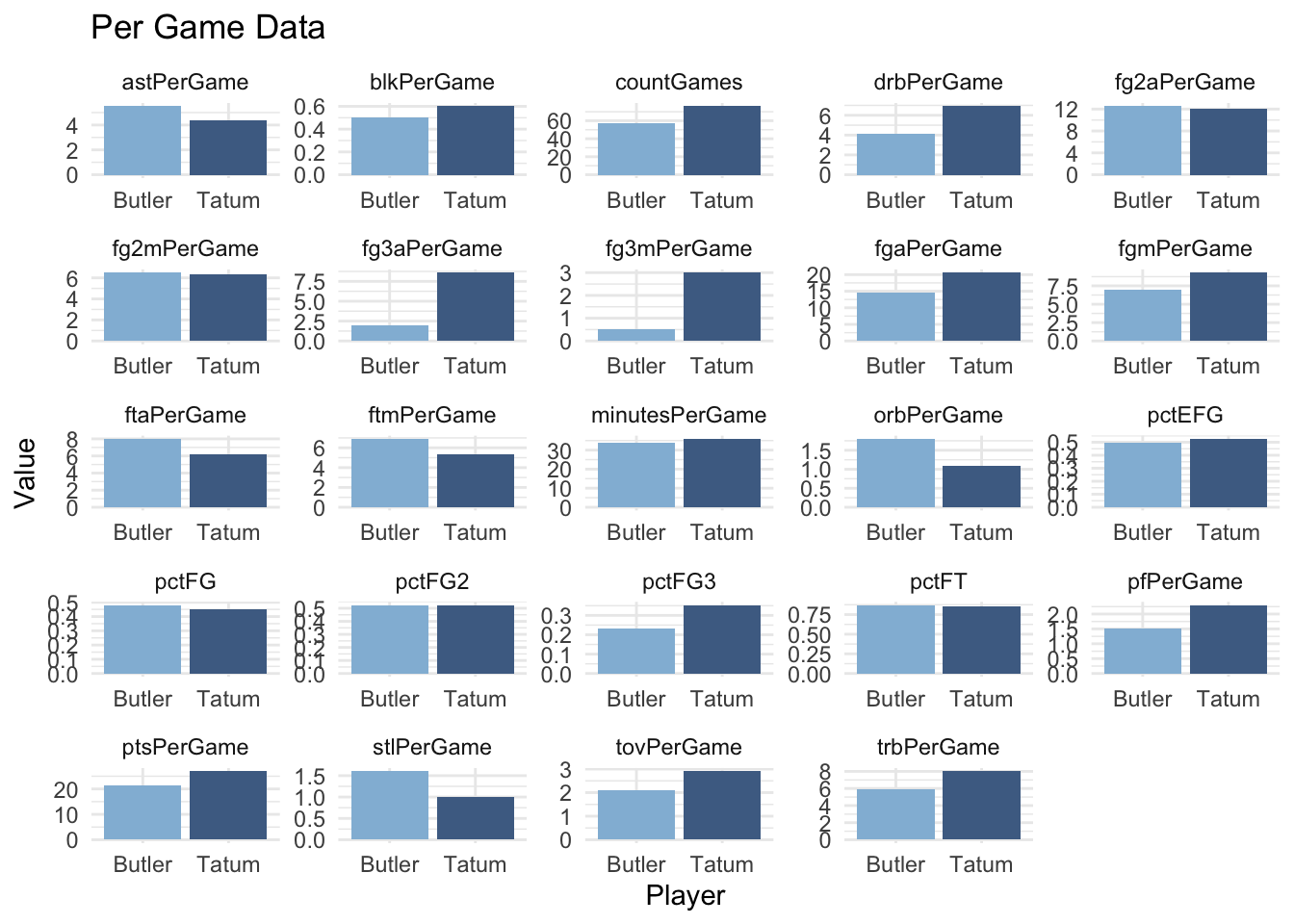
First, let’s compare Jimmy Butler and Jaysom Tatum:
player_comparison(
  player1 = "Jimmy Butler",
  player2 = "Jayson Tatum",
  table = c("per_game", "advanced"),
  season = 2022
)
## parsed http://www.basketball-reference.com/leagues/NBA_2022_per_game.html
## PerGame
## parsed http://www.basketball-reference.com/leagues/NBA_2022_advanced.html
## Advanced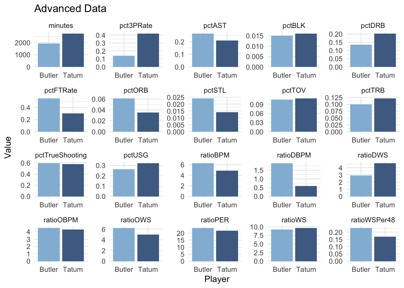
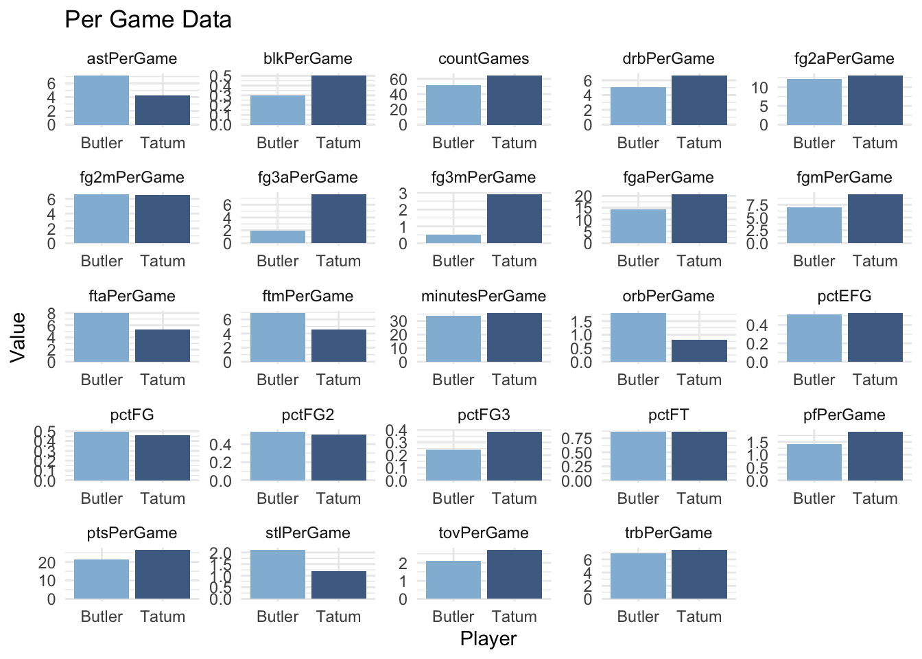
You can even change the year for comparison as long as both players played in that year. Let’s look at 2021:
player_comparison(
  player1 = "Jimmy Butler",
  player2 = "Jayson Tatum",
  table = c("per_game", "advanced"),
  season = 2021
)
## parsed http://www.basketball-reference.com/leagues/NBA_2021_per_game.html
## PerGame
## parsed http://www.basketball-reference.com/leagues/NBA_2021_advanced.html
## Advanced
If you only want the per game statistics do this
player_comparison(
  player1 = "Jimmy Butler",
  player2 = "Jayson Tatum",
  table = c("per_game"),
  season = 2021
)
## PerGame
If you want to have only the advanced statistics do this
player_comparison(
  player1 = "Jimmy Butler",
  player2 = "Jayson Tatum",
  table = c("advanced"),
  season = 2021
)
## Advanced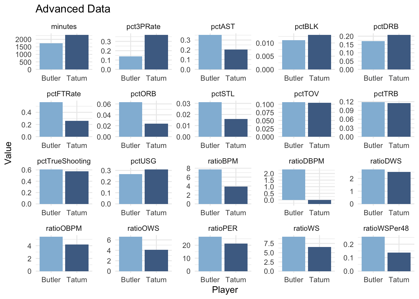
Here’s the code that goes into that function. You can also see it on github here
#load packages
library(nbastatR) #This is for loading NBA data
library(dplyr) #This is for manipulating data sets
library(ggplot2) #This is for graphing data
library(tidyr) # functions for tidying data
library(Hmisc) # loads the %nin% filter
library(ghibli) #for additional colors
#necessary for loading in NBA data
Sys.setenv("VROOM_CONNECTION_SIZE" = 131072 * 2)


player_comparison <- function(
  player1 = "Nikola Jokic",
  player2 = "Joel Embiid",
  table = c("per_game", "advanced"),
  season = 2022
)
{
  player_filter <- c(player1, player2)
  this_data <- vector(mode = "list", length(table)) # initialization

  for (i in 1:length(table)) {
    this_data[[i]] <-
      bref_players_stats(
        seasons = season,
        tables = table[i],
        assign_to_environment = FALSE
      ) %>%
      # Filtering for players
      filter(namePlayer %in% player_filter)
  }

  # Converting data into long format:

  # ADVANCED DATA
  if (sum(table == "advanced")>0) {
    this_index <- which(table == "advanced")

    adv_player_data_long <-
      this_data[[this_index]] %>%
      select(namePlayer, yearSeason, minutes:ratioVORP) %>%
      pivot_longer(cols = c(-namePlayer, -yearSeason)) %>%
      separate(col = namePlayer, into = c("First", "Last"), remove = FALSE)

    adv_player_graphs <-
      ggplot(
        data = adv_player_data_long %>% filter(name%nin%"ratioVORP"),
        aes(x = Last, y = value, fill = namePlayer)
      ) +
      geom_bar(stat = "identity") +
      facet_wrap(~name, scales = "free") +
      labs(title = "Advanced Data", x = "Player", y = "Value") +
      theme_minimal() +
      scale_fill_manual(values = ghibli_palettes$YesterdayMedium[c(4,7)]) +
      theme(legend.position = "none")

    # Prints plot
    print(adv_player_graphs)
  }

  # PER GAME DATA
  if (sum(table == "per_game")>0) {
    this_index <- which(table == "per_game")

    per_player_data_long <-
      this_data[[this_index]] %>%
      select(namePlayer,
             yearSeason,
             countGames,
             pctFG:pctFT,
             minutesPerGame:ptsPerGame) %>%
      pivot_longer(cols = c(-namePlayer, -yearSeason)) %>%
      separate(col = namePlayer, into = c("First", "Last"), remove = FALSE)

    per_player_graphs <-
      ggplot(
        data = per_player_data_long,
        aes(x = Last, y = value, fill = namePlayer)
      ) +
      geom_bar(stat = "identity") +
      facet_wrap(~name, scales = "free") +
      labs(title = "Per Game Data", x = "Player", y = "Value") +
      theme_minimal() +
      scale_fill_manual(values = ghibli_palettes$YesterdayMedium[c(4,7)]) +
      theme(legend.position = "none")

    # Plots graph
    print(per_player_graphs)

  }

}